Weather and My Productivity
Rain or shine affect my mood? Not much.
Weather is often said to affect our mood, and that people in sunnier places are happier because of that. Curious about the possible effect (it could be worth controlling for in my future QS analyses or attempting to imitate benefits inside my house eg. brighter lighting), I combine my long-term daily self-ratings with logs from the nearest major official weather stations, which offer detailed weather information about temperature, humidity, precipitation, cloud cover, wind speed, brightness etc, and try to correlate them.
In general, despite considerable data, there are essentially no bivariate correlations, nothing in several versions of a linear model, and nothing found by a random forest. It would appear that weather does not correlate with my self-ratings to any detectable degree, much less cause it.
Science has found that lighting & temperature & the seasons matter to one’s mood, focus, sleep and other things (but not, apparently, one’s life satisfaction or psychiatric disorders, which may be related to complex features of light ( et al 2014)). Certainly, these things having large effects makes a lot of sense—who doesn’t feel gloomy on a rainy day or happier on a sunny day?
But things everyone knows often turn out to be wrong; and in my case, it seems like my morning use of vitamin D and evening melatonin supplementation may be screening off the environmental effects. So one rainy and then sunny day in March 201312ya, I wondered if I could find an influence of rain or darkness on my own mood or productivity.
As it happens, since 2012-02-16, I have been daily writing down my impression of whether my mood & productivity (MP) that day was average, below-average, or above; this gave me 399 ratings to work with. I didn’t record any weather data, but the nice thing about weather data is that—unlike quotidian but potentially important data like the proverbial what you had for breakfast, which is lost if not immediately recorded—the weather is concrete, objective, easily quantifiable, economically important, and of universal interest. Hence, we would expect weather data to be available online so I can find it, and see what aspects of the weather influence my self-rating (if any).
Data
A convenient source of data seems to be Weather Underground. Going via API is overkill, since we just need data from Islip for 2012-02-16–5m2012-07-0813ya (CSV) and from Pax River 2012-07-11–8m2013-03-2212ya (CSV). I’m using the nearest airport, rather than the nearest volunteer weather station, to get data on cloud cover; cloud cover should be a good proxy for brightness or sunniness. The insol library calculates the length of day, another potentially relevant variable.
# gather and clean data
weather1 <- read.csv("https://www.wunderground.com/history/airport/KISP/2012/2/16/CustomHistory.html?dayend=8&monthend=7&yearend=2012&req_city=NA&req_state=NA&req_statename=NA&format=1")
weather2 <- read.csv("https://www.wunderground.com/history/airport/KNHK/2012/7/11/CustomHistory.html?dayend=29&monthend=7&yearend=2013&req_city=NA&req_state=NA&req_statename=NA&format=1")
weather3 <- read.csv("https://www.wunderground.com/history/airport/KISP/2013/7/30/CustomHistory.html?dayend=7&monthend=8&yearend=2013&req_city=NA&req_state=NA&req_statename=NA&format=1")
weather4 <- read.csv("https://www.wunderground.com/history/airport/KNHK/2013/8/8/CustomHistory.html?dayend=17&monthend=9&yearend=2013&req_city=NA&req_state=NA&req_statename=NA&format=1")

weather1$PrecipitationIn <- as.numeric(as.character(weather1$PrecipitationIn)) # delete weird "T" factor; ???
# mood/productivity (MP) sourced from personal log
weather1$MP <- c(1,3,4,4,4,4,3,4,2,3,4,4,2,3,2,3,3,2,3,2,3,4,3,2,3,2,3,1,2,4,3,3,3,3,3,
                 3,3,2,3,4,3,3,4,4,4,4,2,3,4,3,3,3,4,3,3,1,3,2,3,3,4,3,2,3,2,4,4,4,3,3,
                 4,4,3,4,3,3,2,3,3,2,2,4,3,2,4,4,4,3,3,2,4,4,4,3,3,3,3,2,3,4,3,2,2,4,3,
                 3,2,2,2,2,3,4,2,4,4,3,3,3,2,4,2,2,2,2,2,3,3,4,2,1,3,3,2,3,3,4,2,3,2,3,
                 3,2,4,4)
weather2$MP <- c(2,4,4,4,3,4,3,3,4,3,2,3,4,4,4,3,2,3,3,2,3,3,3,2,2,2,2,2,3,4,3,4,2,4,3,
                 3,2,2,2,3,3,3,3,4,3,3,3,4,3,3,3,2,4,2,3,3,4,4,3,3,3,4,3,3,4,3,4,2,3,3,
                 4,4,3,3,4,4,3,4,3,2,3,3,3,4,3,2,3,2,2,2,3,3,3,4,4,3,4,4,3,3,2,3,3,3,3,
                 4,4,3,4,2,2,2,3,4,3,4,3,4,3,4,4,3,3,2,3,2,4,4,3,4,2,3,4,2,3,3,2,2,2,3,
                 2,3,3,4,2,3,4,3,4,3,3,2,2,3,4,4,3,4,2,2,3,2,3,2,2,2,4,3,3,4,2,2,3,3,3,
                 4,4,3,2,3,2,2,2,3,3,3,4,3,4,3,3,3,2,2,3,3,3,4,4,3,2,2,2,3,3,4,3,4,3,4,
                 3,2,4,4,3,3,2,4,3,3,3,2,3,3,2,3,2,3,3,3,3,2,3,3,3,3,3,3,4,2,3,2,4,3,3,
                 2,2,3,3,3,2,4,3,3,3,3,4,4,3,3,3,3,2,3,2,2,3,3,2,3,2,3,2,3,3,2,2,3,3,3,
                 4,4,3,2,2,3,2,3,2,4,4,4,3,3,3,4,3,4,3,4,4,2,2,2,4,4,3,2,2,3,4,3,2,4,2,
                 3,4,2,4,4,2,3,2,3,3,3,2,2,2,3,3,2,2,3,4,4,2,3,2,2,3,4,4,3,2,2,3,4,4,3,
                 3,3,3,2,4,3,3,4,3,3,3,4,3,4,4,4,4,3,3,3,2,2,2,4,3,4,4,2,2,3,4,4,3,2)
weather3$MP <- c(3,4,2,3,4,3,3,4,3)
weather4$MP <- c(3,3,2,2,3,2,4,4,4,3,2,2,5,4,3,4,4,3,3,4,4,3,2,2,3,4,3,3,4,4,3,4,3,3,
                 4,3,4,4,4,2,3)

# compute length of day for each location
library(insol)
weather1$DayLength <- daylength(40,73, julian(as.Date(as.character(weather1$EDT))), 1)[,3]
weather3$DayLength <- daylength(40,73, julian(as.Date(as.character(weather3$EDT))), 1)[,3]
weather2$DayLength <- daylength(38,76, julian(as.Date(as.character(weather2$EDT))), 1)[,3]
weather4$DayLength <- daylength(38,76, julian(as.Date(as.character(weather4$EDT))), 1)[,3]
# combine & start cleaning
weather <- rbind(weather1,weather2)
weather$WindDirDegrees.br... <- sub("<br />", "", weather$WindDirDegrees.br...)
weather$WindDirDegrees.br... <- as.integer(weather$WindDirDegrees.br...)
weather$Events <- as.integer(weather$Events)
weather$Events[weather$Events>1] <- 2
# something of a hack but we'll impute any missing rain precipitation values as 0
weather[is.na(weather)] <- 0
Analysis
Exploratory
After cleanup, the data looks reasonable and as expected, with each variable spanning the ranges one would expect of temperatures and precipitation:
summary(weather)
#         EDT      Max.TemperatureF Mean.TemperatureF Min.TemperatureF Max.Dew.PointF MeanDew.PointF
#  2012-2-16:  1   Min.   : 26.0    Min.   :21.0      Min.   :14.0     Min.   :12.0   Min.   : 1
#  2012-2-17:  1   1st Qu.: 53.0    1st Qu.:45.0      1st Qu.:37.0     1st Qu.:39.8   1st Qu.:33
#  2012-2-18:  1   Median : 68.0    Median :58.0      Median :50.0     Median :54.0   Median :48
#  2012-2-19:  1   Mean   : 66.9    Mean   :58.7      Mean   :50.6     Mean   :52.5   Mean   :47
#  2012-2-20:  1   3rd Qu.: 82.0    3rd Qu.:73.0      3rd Qu.:66.0     3rd Qu.:67.0   3rd Qu.:63
#  2012-2-21:  1   Max.   :100.0    Max.   :87.0      Max.   :80.0     Max.   :79.0   Max.   :74
#  (Other)  :522
#  Min.DewpointF   Max.Humidity   Mean.Humidity   Min.Humidity  Max.Sea.Level.PressureIn
#  Min.   :-5.0   Min.   : 42.0   Min.   :28.0   Min.   :12.0   Min.   :29.4
#  1st Qu.:25.0   1st Qu.: 82.0   1st Qu.:59.0   1st Qu.:37.0   1st Qu.:30.0
#  Median :42.0   Median : 89.0   Median :69.0   Median :48.0   Median :30.1
#  Mean   :41.2   Mean   : 85.7   Mean   :67.8   Mean   :48.6   Mean   :30.1
#  3rd Qu.:58.0   3rd Qu.: 93.0   3rd Qu.:77.2   3rd Qu.:60.0   3rd Qu.:30.2
#  Max.   :73.0   Max.   :100.0   Max.   :97.0   Max.   :93.0   Max.   :30.6
#
#  Mean.Sea.Level.PressureIn Min.Sea.Level.PressureIn Max.VisibilityMiles Mean.VisibilityMiles
#  Min.   :29.1              Min.   :28.7             Min.   : 6.00       Min.   : 2.0
#  1st Qu.:29.9              1st Qu.:29.8             1st Qu.:10.00       1st Qu.: 9.0
#  Median :30.0              Median :29.9             Median :10.00       Median :10.0
#  Mean   :30.0              Mean   :29.9             Mean   : 9.97       Mean   : 9.1
#  3rd Qu.:30.2              3rd Qu.:30.1             3rd Qu.:10.00       3rd Qu.:10.0
#  Max.   :30.5              Max.   :30.5             Max.   :10.00       Max.   :10.0
#
#  Min.VisibilityMiles Max.Wind.SpeedMPH Mean.Wind.SpeedMPH Max.Gust.SpeedMPH PrecipitationIn
#  Min.   : 0.00       Min.   : 6.0      Min.   : 1.00      Min.   : 0.0      Min.   :0.000
#  1st Qu.: 3.00       1st Qu.:13.0      1st Qu.: 6.00      1st Qu.: 0.0      1st Qu.:0.000
#  Median : 9.00       Median :15.0      Median : 8.00      Median :22.0      Median :0.000
#  Mean   : 6.88       Mean   :16.4      Mean   : 8.04      Mean   :18.6      Mean   :0.124
#  3rd Qu.:10.00       3rd Qu.:20.0      3rd Qu.:10.00      3rd Qu.:28.0      3rd Qu.:0.030
#  Max.   :10.00       Max.   :40.0      Max.   :27.00      Max.   :56.0      Max.   :6.000
#
#    CloudCover      Events     WindDirDegrees.br...       MP         DayLength
#  Min.   :0.0   Min.   :1.00   Min.   :  1          Min.   :1.00   Min.   : 9.27
#  1st Qu.:3.0   1st Qu.:1.00   1st Qu.:138          1st Qu.:2.00   1st Qu.:10.31
#  Median :4.5   Median :1.00   Median :208          Median :3.00   Median :12.10
#  Mean   :4.4   Mean   :1.47   Mean   :202          Mean   :2.98   Mean   :12.07
#  3rd Qu.:6.0   3rd Qu.:2.00   3rd Qu.:283          3rd Qu.:4.00   3rd Qu.:13.87
#  Max.   :8.0   Max.   :2.00   Max.   :360          Max.   :4.00   Max.   :14.73
CloudCover being 0–8 looks a bit odd, since one might’ve expected a decimal or percentage or some quantification of thickness but turns out to be a standard measurement, the “okta”. We might expect some seasonal effects, but graphing a sensitive LOESS moving average and then a per-week spineplot suggests just 1 anomaly, that there were some days I rated “1” but never subsequently (this has an explanation: as I began keeping the series, my car caught on fire, was totaled; and I was then put through the wringer with the insurance & junkyard, and felt truly miserable at multiple points):
par(mfrow=c(2,1))
scatter.smooth(x=weather$EDT, y=weather$MP, span=0.3, col="#CCCCCC", xlab="Days", ylab="MP rating")
weeks <- c(seq(from=1,to=length(weather$MP),by=7), length(weather$MP))
spineplot(c(1:(length(weather$MP))), as.factor(weather$MP), breaks=weeks, xlab="Weeks", ylab="MP rating ratios")
# we don't use the date past the spineplot &
# it causes problems with all the models, so delete it
rm(weather$EDT)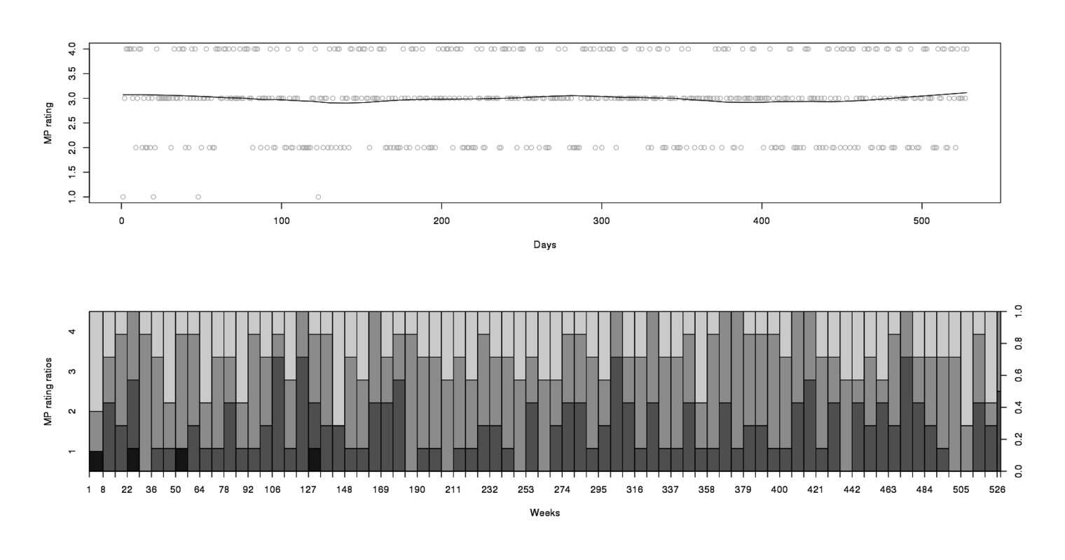
MP from February 201213ya to March 2013
A formal check for autocorrelation in MP ratings (most methods assume independence) turns up little enough that I feel free to ignore them. So the data looks clean and tame; now we can begin real interpretation. The first and most obvious thing to do is to see what the overall correlation matrix with MP looks like:
# all weather correlations with mood/productivity
round(cor(weather)[23,], digits=3)
#          Max.TemperatureF         Mean.TemperatureF          Min.TemperatureF
#                     0.013                     0.016                     0.022
#            Max.Dew.PointF            MeanDew.PointF             Min.DewpointF
#                     0.016                     0.019                     0.016
#              Max.Humidity             Mean.Humidity              Min.Humidity
#                     0.042                     0.026                     0.011
#  Max.Sea.Level.PressureIn Mean.Sea.Level.PressureIn  Min.Sea.Level.PressureIn
#                     0.006                     0.004                     0.015
#       Max.VisibilityMiles      Mean.VisibilityMiles       Min.VisibilityMiles
#                     0.066                     0.004                    -0.016
#         Max.Wind.SpeedMPH        Mean.Wind.SpeedMPH         Max.Gust.SpeedMPH
#                     0.008                     0.002                     0.018
#           PrecipitationIn                CloudCover                    Events
#                    -0.037                     0.041                    -0.001
#      WindDirDegrees.br...                        MP                 DayLength
#                    -0.006                     1.000                     0.036
# tail(sort(abs(round(cor(weather)[23,], digits=3))), 6)
#           DayLength     PrecipitationIn          CloudCover        Max.Humidity Max.VisibilityMiles
#               0.036               0.037               0.041               0.042               0.066
#                  MP
#               1.000
All the r values seem very small: >0.1. But some of the more plausible correlations may be statistically-significant, so we’ll look at the 5 largest correlations
sapply(c("DayLength","PrecipitationIn","CloudCover","Max.Humidity","Max.VisibilityMiles"),
       function(x) cor.test(weather$MP, weather[[x]]))
# ...
#             DayLength                              PrecipitationIn
# p.value     0.4099                                 0.394
# estimate    0.03594                                -0.03717
#
#             CloudCover                             Max.Humidity
# p.value     0.3445                                 0.3319
# estimate    0.04122                                0.04231
#
#             Max.VisibilityMiles
# p.value     0.1292
# estimate    0.06611
These specific variables turn out to be failures too, with large p-values.
One useful technique is to convert metrics into standardized units (of standard deviations), sum them all into a single composite variable, and then test that; this can reveal influences not obvious if one looked at the metrics individually. (For example, in my potassium sleep experiments, where I was interested in an overall measure of reduced sleep quality rather than single metrics like sleep latency.) Perhaps this would work here?
# construct a z-score for all of them to see if it does any better
with(weather, cor.test(MP, (scale(Max.Humidity) + scale(Max.VisibilityMiles)
                            + scale(PrecipitationIn) + scale(CloudCover) + scale(DayLength))))
# ...
# t = 1.296, df = 526, p-value = 0.1957
# alternative hypothesis: true correlation is not equal to 0
# 95% confidence interval:
#  -0.02908  0.14105
# sample estimates:
#    cor
# 0.0564
Modeling
Continuous MP
Linear Model
Touji: “Oh, yes. the view of the world that one can have is quite small.”
Hikari: “Yes, you measure things only by your own small measure.”
Asuka: “One sees things with the truth, given by others.”
Misato: “Happy on a sunny day.”
Rei: “Gloomy on a rainy day.”
Asuka: “If you’re taught that, you always think so.”
Ritsuko: “But, you can enjoy rainy days.”Neon Genesis Evangelion, episode 26 “The Beast that Shouted ‘I’ at the Heart of the World” (Literal Translation Project)
The correlations show individually little value, so we’ll move on to building modeling and assessing their fit. Can we accurately predict MP if we use all the parameters? We’ll start with a linear model/regression, where we treat the categorical MP variable as a continuous variable for simplicity:
model1 <- lm(MP ~ ., data=weather); summary(model1)
# ...Residuals:
#     Min      1Q  Median      3Q     Max
# -2.0255 -0.7815  0.0165  0.8126  1.3730
#
# Coefficients:
#                            Estimate Std. Error t value Pr(>|t|)
# (Intercept)               -4.29e+00   6.38e+00   -0.67     0.50
# Max.TemperatureF           3.76e-02   3.20e-02    1.17     0.24
# Mean.TemperatureF         -5.87e-02   6.06e-02   -0.97     0.33
# Min.TemperatureF           4.41e-02   3.24e-02    1.36     0.17
# Max.Dew.PointF            -9.52e-03   1.46e-02   -0.65     0.52
# MeanDew.PointF            -1.45e-02   2.79e-02   -0.52     0.60
# Min.DewpointF             -6.52e-03   1.43e-02   -0.46     0.65
# Max.Humidity               1.10e-02   8.36e-03    1.31     0.19
# Mean.Humidity              1.73e-03   1.33e-02    0.13     0.90
# Min.Humidity               5.75e-03   8.16e-03    0.71     0.48
# Max.Sea.Level.PressureIn   9.92e-01   9.79e-01    1.01     0.31
# Mean.Sea.Level.PressureIn -1.61e+00   1.63e+00   -0.99     0.32
# Min.Sea.Level.PressureIn   7.29e-01   8.39e-01    0.87     0.39
# Max.VisibilityMiles        2.00e-01   1.47e-01    1.36     0.17
# Mean.VisibilityMiles       1.04e-02   3.96e-02    0.26     0.79
# Min.VisibilityMiles       -3.94e-03   1.89e-02   -0.21     0.83
# Max.Wind.SpeedMPH          2.31e-03   1.32e-02    0.18     0.86
# Mean.Wind.SpeedMPH        -2.28e-03   1.70e-02   -0.13     0.89
# Max.Gust.SpeedMPH          2.71e-03   4.54e-03    0.60     0.55
# PrecipitationIn           -1.25e-01   9.29e-02   -1.35     0.18
# CloudCover                 2.65e-02   2.53e-02    1.05     0.29
# Events                    -9.18e-02   9.83e-02   -0.93     0.35
# WindDirDegrees.br...       3.08e-05   4.11e-04    0.07     0.94
# DayLength                  5.72e-02   4.78e-02    1.20     0.23
#
# Residual standard error: 0.755 on 504 degrees of freedom
# Multiple R-squared:  0.0282,    Adjusted R-squared:  -0.0162
# F-statistic: 0.635 on 23 and 504 DF,  p-value: 0.905
The variance explained is extremely minimal, even with 23 different variables in the linear model, and suggests overfitting (as one would expect). By Occam’s razor, most of the variables should be scrapped for not carrying their weight; the step function uses a complexity penalty to choose which variable to eliminate while still fitting the data reasonably well. It choose to keep only 4 variables:
smodel1 <- step(model1); summary(smodel1)
# ...Residuals:
#     Min      1Q  Median      3Q     Max
# -2.1301 -0.8907  0.0121  0.8990  1.1779
#
# Coefficients:
#                     Estimate Std. Error t value Pr(>|t|)
# (Intercept)          0.02134    1.38025    0.02    0.988
# Min.TemperatureF     0.01429    0.01008    1.42    0.157
# MeanDew.PointF      -0.01489    0.01034   -1.44    0.150
# Max.Humidity         0.00958    0.00531    1.81    0.072
# Max.VisibilityMiles  0.21250    0.12682    1.68    0.094
#
# Residual standard error: 0.748 on 523 degrees of freedom
# Multiple R-squared:  0.0109,    Adjusted R-squared:  0.00336
# F-statistic: 1.44 on 4 and 523 DF,  p-value: 0.218
We can compare the models’ prediction accuracy on the dataset (lower is better in mean-squared-error):
mean((weather$MP - weather$MP)^2) # perfect
# [1] 0
mean((weather$MP - model1$fitted.values)^2) # original
# [1] 0.5446
mean((weather$MP - smodel1$fitted.values)^2) # much simpler model
# [1] 0.5543
model2 <- lm(MP ~ 1, data=weather); mean((weather$MP - model2$fitted.values)^2)
# [1] 0.5604
The model with 4 data variables is much simpler, and appears to fit almost as well, but slightly better than the null model of no parameters
Random Forests Regression
Linear modeling having failed to reveal any interesting relationships, we’ll take one last crack at it: if there’s any interesting predictive power in the weather data at all, a high-powered machine learning technique like random forests ought to build a model which outperforms the linear model at least a little on mean-squared-error
library(randomForest)
rmodel <- randomForest(MP ~ ., data=weather, proximity=TRUE); rmodel
# ...
#                Type of random forest: regression
#                      Number of trees: 500
# No. of variables tried at each split: 7
#
#           Mean of squared residuals: 0.5692
#                     % Var explained: -1.57
The error with all variables is a little higher than the simpler linear model. Troublingly, a random forests with the 4 simpler variables increases the error:
srmodel <- randomForest(MP ~ Min.TemperatureF + MeanDew.PointF + Max.Humidity + Max.VisibilityMiles, data=weather, proximity=TRUE); srmodel
# ...
#                Type of random forest: regression
#                      Number of trees: 500
# No. of variables tried at each split: 1
#
#           Mean of squared residuals: 0.5814
#                     % Var explained: -3.76
Perhaps treating MP as a continuous variable was a bad idea. Let’s start over.
Categorical MP
We turn the MP data into an ordered factor:
weather$MP <- ordered(weather$MP)Logistic Model
A straight logistic regression (glm(MP ~ ., data=weather, family="binomial")) is not appropriate because MP is not a binary outcome; we use the MASS library to do an ordinal logistic regression; as with the linear model, the coefficients don’t seem to differ very much
library(MASS)
lmodel <- polr(as.ordered(MP) ~ ., data = weather); summary(lmodel)
# ...
# Coefficients:
#                               Value Std. Error t value
# Max.TemperatureF           0.086798    0.07916   1.096
# Mean.TemperatureF         -0.135828    0.14974  -0.907
# Min.TemperatureF           0.105068    0.08024   1.309
# Max.Dew.PointF            -0.023466    0.03624  -0.648
# MeanDew.PointF            -0.033449    0.06789  -0.493
# Min.DewpointF             -0.018700    0.03424  -0.546
# Max.Humidity               0.029043    0.02036   1.427
# Mean.Humidity              0.004063    0.03263   0.124
# Min.Humidity               0.013462    0.02024   0.665
# Max.Sea.Level.PressureIn   2.554493    0.85951   2.972
# Mean.Sea.Level.PressureIn -4.352709    0.06383 -68.191
# Min.Sea.Level.PressureIn   2.047343    0.91077   2.248
# Max.VisibilityMiles        0.549889    0.37650   1.461
# Mean.VisibilityMiles       0.029195    0.09772   0.299
# Min.VisibilityMiles       -0.007733    0.04638  -0.167
# Max.Wind.SpeedMPH          0.003846    0.03219   0.119
# Mean.Wind.SpeedMPH        -0.007351    0.04250  -0.173
# Max.Gust.SpeedMPH          0.008375    0.01130   0.741
# PrecipitationIn           -0.325188    0.22738  -1.430
# CloudCover                 0.067914    0.06000   1.132
# Events                    -0.219315    0.24050  -0.912
# WindDirDegrees.br...       0.000192    0.00101   0.190
# DayLength                  0.144132    0.11804   1.221
#
# Intercepts:
#     Value   Std. Error t value
# 1|2  13.143   0.021    638.830
# 2|3  17.080   0.500     34.185
# 3|4  19.126   0.509     37.550
#
# Residual Deviance: 1143.49
# AIC: 1195.49
## relative risk or odds; how much difference does each variable make, per its units?
exp(coef(lmodel))
#          Max.TemperatureF         Mean.TemperatureF          Min.TemperatureF
#                   1.09068                   0.87299                   1.11079
#            Max.Dew.PointF            MeanDew.PointF             Min.DewpointF
#                   0.97681                   0.96710                   0.98147
#              Max.Humidity             Mean.Humidity              Min.Humidity
#                   1.02947                   1.00407                   1.01355
#  Max.Sea.Level.PressureIn Mean.Sea.Level.PressureIn  Min.Sea.Level.PressureIn
#                  12.86477                   0.01287                   7.74729
#       Max.VisibilityMiles      Mean.VisibilityMiles       Min.VisibilityMiles
#                   1.73306                   1.02963                   0.99230
#         Max.Wind.SpeedMPH        Mean.Wind.SpeedMPH         Max.Gust.SpeedMPH
#                   1.00385                   0.99268                   1.00841
#           PrecipitationIn                CloudCover                    Events
#                   0.72239                   1.07027                   0.80307
#      WindDirDegrees.br...                 DayLength
#                   1.00019                   1.15504
Another use of step; this time, it builds something even narrower than before:
slmodel <- step(lmodel); summary(slmodel)
# ...Coefficients:
#                     Value Std. Error t value
# Max.VisibilityMiles 0.527      0.329     1.6
#
# Intercepts:
#     Value Std. Error t value
# 1|2 0.364 3.293      0.110
# 2|3 4.277 3.282      1.303
# 3|4 6.283 3.287      1.912
#
# Residual Deviance: 1156.46
# AIC: 1164.46
exp(0.527)
# [1] 1.694
Seasonal Effects
The previously mentioned life-satisfaction/weather paper, Lucas et al 201312ya, examined a single variable very similar to my MP:
Life satisfaction was assessed using a single item that read, “In general, how satisfied are you with your life.” Participants responded using a 4-point scale with the options “Very Satisfied,” “Satisfied,” “Dissatisfied,” or “Very Dissatisfied” (responses were scored such that higher scores reflect higher satisfaction)
Rather than simply regress local weather on the score, similar to what I’ve been doing so far, they attempted a more complex model where the effects could change based on region & time of year:
In addition, the effect of absolute levels of any weather variable may vary depending on when in the year the weather occurred. A 50℉ day may contribute to positive mood (and hence higher life satisfaction) if it occurred in the middle of winter in a cold climate, whereas this same absolute temperature might contribute to a negative mood (and hence lower life satisfaction) if it occurred in the middle of summer in a warm climate. Thus, seasonal differences must be considered when examining the effects of weather.
While I live in only one region and replicating the rest of the analysis would be a lot of work, the seasonal changes is possible and not too hard to investigate: reset the data to restore the date, create a Season variable, populate (since I am lazy, I convert the dates to fiscal quarters, which are similar enough), and then rerun an ordinal logistic regression with all the potential predictors nested under Season.
Looking at the coefficients split by season, and looking for coefficients that suddenly become larger or which switch signs from season to season, I see no real candidates:
weather$MP <- as.ordered(weather$MP)
library(lubridate)
weather$Season <- quarter(weather$EDT)
library(lme4)
lmr <- lmer(MP ~ (. |Season), data=weather, control = lmerControl(maxfun=20000)); ranef(lmr)
# ...$Season
#   (Intercept)   MP.L   MP.Q    MP.C       EDT Max.TemperatureF Mean.TemperatureF Min.TemperatureF
# 1     0.05723 1.8727 0.2184 -0.1058 4.704e-05         0.002089         -0.002253        0.0009085
# 2     0.06215 1.8918 0.2303 -0.1042 6.786e-06         0.004284         -0.004817        0.0034466
# 3     0.31806 0.9037 0.9451 -0.4151 3.206e-05         0.003028         -0.002113        0.0019708
# 4     0.31525 0.8986 0.9376 -0.4169 7.582e-07        -0.001217         -0.001045        0.0003388
#   Max.Dew.PointF MeanDew.PointF Min.DewpointF Max.Humidity Mean.Humidity Min.Humidity
# 1     -3.416e-04      -0.002731     0.0008853   -1.584e-04     0.0015697    0.0004101
# 2      1.922e-03      -0.004427     0.0001578    6.227e-04    -0.0002743    0.0010211
# 3      2.523e-05      -0.002938    -0.0007302    5.611e-05     0.0009317    0.0004772
# 4     -1.235e-04       0.003389    -0.0012974    6.986e-04    -0.0009484   -0.0004437
#   Max.Sea.Level.PressureIn Mean.Sea.Level.PressureIn Min.Sea.Level.PressureIn Max.VisibilityMiles
# 1                 0.006218                 -0.018023                -0.008160            0.013916
# 2                 0.011742                 -0.001504                 0.001079           -0.002815
# 3                 0.002675                  0.002821                -0.004279            0.005178
# 4                 0.006987                  0.003645                 0.007091            0.013030
#   Mean.VisibilityMiles Min.VisibilityMiles Max.Wind.SpeedMPH Mean.Wind.SpeedMPH Max.Gust.SpeedMPH
# 1            -0.002323           0.0028401         0.0028779          0.0009989        -6.320e-04
# 2             0.001611          -0.0023890         0.0014840         -0.0012118        -7.029e-05
# 3             0.002107           0.0007576        -0.0014126         -0.0016919         9.457e-04
# 4            -0.006157           0.0020409         0.0007483          0.0008237        -4.648e-04
#   PrecipitationIn CloudCover    Events WindDirDegrees.br... DayLength   Season.L Season.Q
# 1       -0.025717   0.002471  0.005752            1.576e-05  0.009140 -0.0006296 0.005954
# 2       -0.005913  -0.002430 -0.002981           -1.195e-04 -0.003607 -0.0015844 0.006389
# 3        0.002764   0.003450 -0.006076            6.861e-06 -0.004650 -0.0011383 0.010232
# 4       -0.008745   0.002082 -0.012127           -4.119e-05  0.003976 -0.0010785 0.010584
#     Season.C
# 1 -0.0041696
# 2 -0.0047106
# 3 -0.0011607
# 4 -0.0004978
Variables which are positive in one season tend to be positive in another. There are some cases of flipping sign, like PrecipitationIn but in these cases, the coefficients are tiny (sometimes so tiny R lapses into scientific notation). In no case is the difference between season estimates as large as 0.1. Hence, seasonal effects do not seem to be important
Correlation Size & Implications
The Max.VisibilityMiles result seems like a reasonable one; the variable may be tapping into some sort of anti-rain measure. We can visualize the coefficients thusly:
library(arm)
maxvis <- attr(profile(slmodel), "summary")$coefficients[1]
coefplot(maxvis, varnames=rownames(x), vertical=FALSE, var.las=1, main="95% CIs for the log odds of predictors")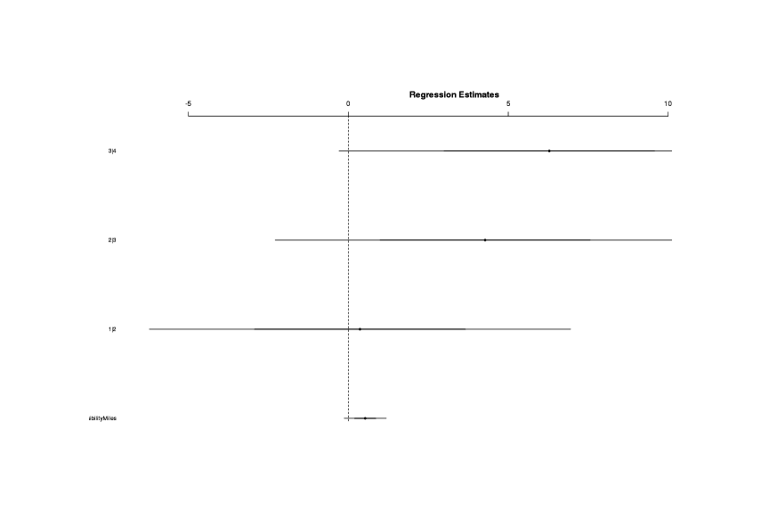
Variables with confidence intervals show log odds size and whether the CI excludes zero
It doesn’t look particularly impressive and doesn’t exclude 0; but we want to know whether this surviving variable is potentially useful in practice, what its “cash value” might be. We again exponentiate the log odds to get more understandable odds:
exp(coef(slmodel))
# Max.VisibilityMiles
#              1.694
What do these estimates mean in practice? Let’s take Max VisibilityMiles as a variable that may be manipulable by buying bright lights, with an odds of 1.5; if we could somehow maximize each day’s DayLength, the model would predict 4 higher days:
weatherOdds <- weather # copy data & max out DayLength
weatherOdds$Max.VisibilityMiles <- max(weather$Max.VisibilityMiles)
sum(as.integer(predict(slmodel, newdata=weatherOdds))) - sum(as.integer(predict(slmodel, newdata=weather)))
# [1] 4
If we wanted to test this potential effect via an experiment (eg. buying a powerful lighting system, and turning it on or off on random days), how many days n should the experiment run? With a bootstrap: we can calculate the effect size of 4 incremented days and then ask for the n required for a self-experiment with good power of 80%; this turns out to be a ~1600 day or 4.4 year long experiment:
library(boot)
library(rms)
n <- 1600
weatherPower <- function(dt, indices) {
    d <- dt[sample(nrow(dt), n, replace=TRUE), ] # new dataset, possibly larger than the original
    lmodel <- lrm(MP ~ Max.VisibilityMiles, data = d)
    return(anova(lmodel)[5])
}
bs <- boot(data=weather, statistic=weatherPower, R=100000, parallel="multicore", ncpus=4)
alpha <- 0.05
print(sum(bs$t<=alpha)/length(bs$t))
# [1] 0.8054
To detect such a subtle effect is not easy, and such a time-consuming experiment is surely not worthwhile.
Random Forests Classification
Random forests can be used to classify (predict categorical outcomes) as well as regressions; having turned the response variable into a factor, the type switches automatically:
rmodel <- randomForest(MP ~ ., data=weather, proximity=TRUE); rmodel
# ...
#                      Number of trees: 500
# No. of variables tried at each split: 4
#
#         OOB estimate of  error rate: 57.39%
# Confusion matrix:
#   1  2   3  4 class.error
# 1 0  1   3  0      1.0000
# 2 0 20 104 16      0.8571
# 3 0 31 179 34      0.2664
# 4 0 20  94 26      0.8143
We can’t step through random forests since it doesn’t have a complexity measure like AIC to use, so we’ll reuse the variable from the simplified ordinal:
srmodel <- randomForest(MP ~ Max.VisibilityMiles, data=weather, proximity=TRUE); srmodel
# ...
#                Type of random forest: classification
#                      Number of trees: 500
# No. of variables tried at each split: 1
#
#         OOB estimate of  error rate: 53.79%
# Confusion matrix:
#   1 2   3 4 class.error
# 1 0 0   4 0    1.000000
# 2 0 2 138 0    0.985714
# 3 0 1 242 1    0.008197
# 4 0 0 140 0    1.000000
Much better, and now slightly better than the original linear models.
Ordinal vs Random Forests
We can now compare the fraction of days that are incorrectly predicted by the constant predictor, the ordinal logistic regression (full & simplified), and the random forests (full & simplified):
1 - (sum(weather$MP==3) / length(weather$MP))
# [1] 0.5379
1 - (sum(weather$MP == as.integer(predict(lmodel))) / length(weather$MP))
# [1] 0.5284
1 - (sum(as.integer(weather$MP) == predict(slmodel)) / length(weather$MP))
# [1] 0.5341

1 - (sum(as.integer(weather$MP) == as.integer(predict(rmodel))) / length(weather$MP))
# [1] 0.5739
1 - (sum(as.integer(weather$MP) == as.integer(predict(srmodel))) / length(weather$MP))
# [1] 0.5379
It would seem that there is no big difference between the models, but the ordinal may be a little bit better than the constant predictor.
Model Checking
Error Rate
Before concluding that the ordinal logistic regression is better than the constant predictor, it might be a good idea to check how robust this result holds up. The difference in correctly classified days is very small, and it might represent minimal advantage. We’ll bootstrap a large number of logistic regressions on samples of the full dataset, and see what fraction of them incur a higher classification error rate than the constant predictor:
library(boot)
errorRate <- function(dt, indices) {
  d <- dt[indices,] # allows boot to select subsample
  lmodel <- polr(as.ordered(MP) ~ ., data = d) # train new regression model on subsample
  return(1 - (sum(d$MP == as.integer(predict(lmodel))) / length(d$MP)))
}
bs <- boot(data=weather, statistic=errorRate, R=100000, parallel="multicore", ncpus=4); bs
# ...Bootstrap Statistics :
#     original   bias    std. error
# t1*   0.5284 -0.01137     0.02431

boot.ci(bs)
# ...
# Intervals :
# Level      Normal              Basic
# 95%   ( 0.4921,  0.5874 )   ( 0.4905,  0.5871 )
#
# Level     Percentile            BCa
# 95%   ( 0.4697,  0.5663 )   ( 0.4905,  0.5890 )


hist(bs$t, xlab="Error rate", ylab="Number of samples",
           main="Bootstrap check of ordinal logistic regression accuracy")
sum(bs$t > (1 - (sum(weather$MP==3) / length(weather$MP)))) / length(bs$t)
# [1] 0.1832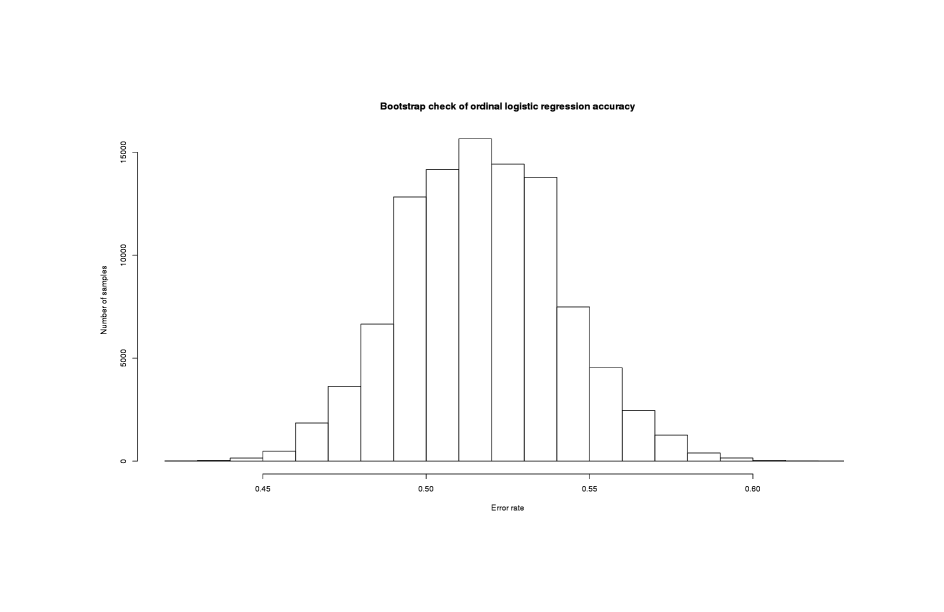
Distribution of logistic regression classification rates
There’s substantial uncertainty in the classification rate, as evidenced by the potentially wide confidence intervals, but in ~18% of the new logistic regressions, the classification rate was worse than the constant predictor. This is not too bad but the logistic regression is not outperforming random by very much, so the reality of the result is open to question.
Conclusion
An attack on the data turned up nothing in several ways; the only model that seemed to improve on random guessing does not do so by very much, indicating weak weather effects. I will attempt to follow up in 2 years to see if the results replicate with a longer data series.
Appendix
Autocorrelation
A test using acf shows no autocorrelation worth mentioning:
acf(weather$MP, main="Do days predict subsequent days at various distances?")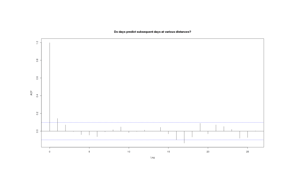
MP series shows almost no autocorrelation at any timelag
For comparison, here is acf for a data series where one would expect a great deal of autocorrelation—my daily weight 2012–201312ya—and one does indeed observe it:
weight <- c(205,214,216,213,213,218,218,214,215,216,218,216,210,219,217,219,217,215,215,217,219,
    216,215,218,215,219,219,219,218,218,220,220,219,219,219,221,220,219,216,220,220,218,
    218,220,219,220,215,215,218,218,215,216,216,218,218,220,219,216,217,220,215,215,218,
    216,214,213,216,215,214,213,214,216,216,212,209,212,214,213,210,211,210,213,211,215,
    211,212,212,216,212,215,216,215,215,212,216,213,212,211,215,214,215,216,214,212,212,
    213,212,213,211,214,215,210,211,211,211,212,210,210,212,211,214,213,214,212,215,214,
    213,215,211,214,214,216,215,213,215,213,213,212,215,211,212,212,211,212,211,212,210,
    211,213,218,217,212,214,216,213,212,211,211,214,212,211,216,NA,NA,NA,NA,NA,218,
    216,214,215,216,216,213,216,214,215,219,218,216,215,218,217,219,219,219,219,219,218,
    217,216,216,215,218,219,217,216,219,217,216,216,219,216,218,215,216,215,215,213,214,
    215,217,216,215,215,216,214,215,215,214,216,211,214,213,214,211,212,211,210,212,211,
    212,214,212,211,214,212,211,212,211,212,213,210,212,210,210,211,210,212,210,210,210,
    210,210,209,206,206,208,209,207,207,205,205,205,206,206,209,204,206,206,204,204,204,
    204,205,203,205,203,205,204,204,203,204,204,205,205,204,205,205,204,204,205,205,205,
    205,204,203,205,205,206,205,204,203,204,205,206,207,206,205,205,207,206,210,210,212,
    211,208,210,210,209,211,212,204,205,208,208,209,209,208,208,208,209,208,210,209,208,
    207,207,209,208,209,207,207,206,207,208,207,209,210,210,208,208,206,208,210,210,209,
    209,209,210,209,210,212,212,210,212,213,NA,NA,NA,NA,NA,NA,NA,NA,NA,NA,210,
    211,210,210,210,211,212,211,210,210,210,212,210,211,210,209,211,209,209,210,210,210,
    211,210,210,209,213,210,210,210,214,212,211,210,211,215,215,214,210,214,212)
acf(weight, na.action = na.pass)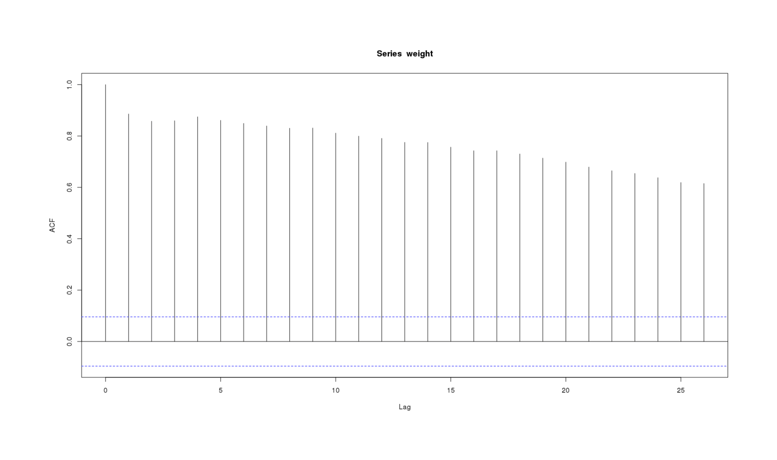
Weight series showing autocorrelation at every timelag